Fullerének és szén nanocsövek előadás fizikus és vegyész hallgatóknak (2011 tavaszi félév – április 4.) Kürti Jenő Koltai János (helyettesítés) ELTE Biológiai.

Az előadások a következő témára: "Fullerének és szén nanocsövek előadás fizikus és vegyész hallgatóknak (2011 tavaszi félév – április 4.) Kürti Jenő Koltai János (helyettesítés) ELTE Biológiai."— Előadás másolata:

1 Fullerének és szén nanocsövek előadás fizikus és vegyész hallgatóknak (2011 tavaszi félév – április 4.) Kürti Jenő Koltai János (helyettesítés) ELTE Biológiai Fizika Tanszék

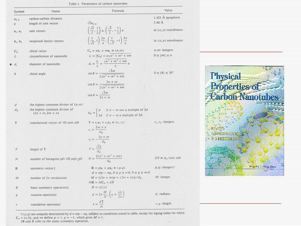
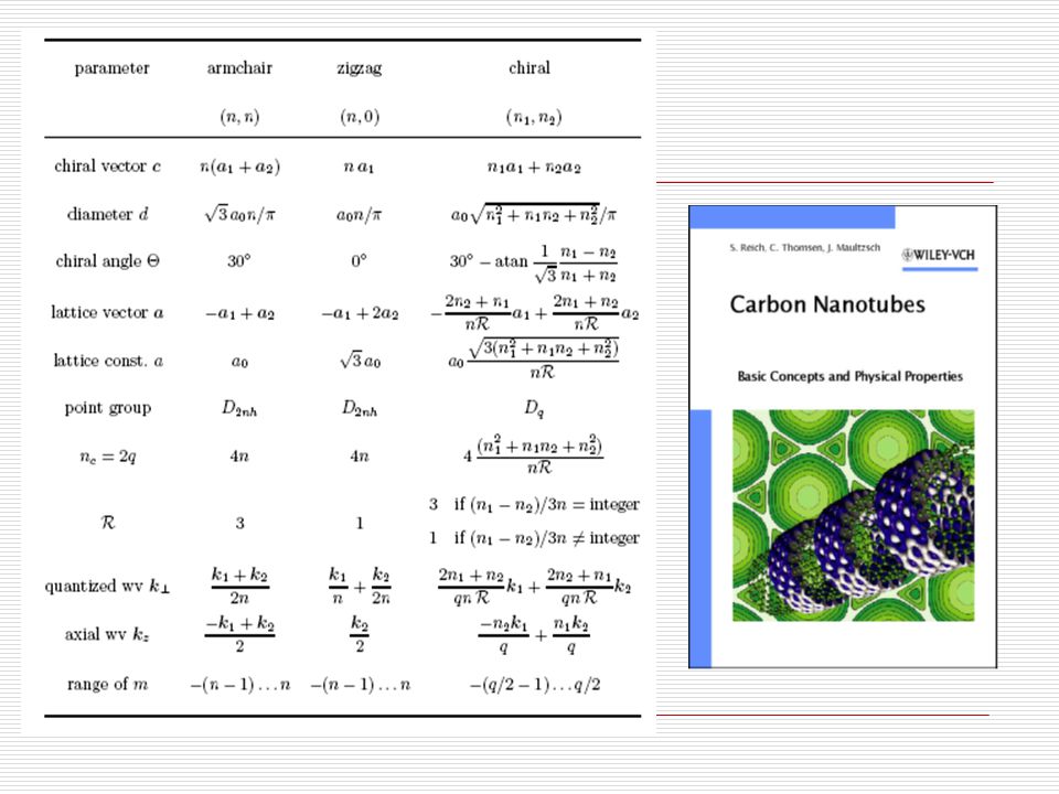
2 C h = n·a 1 +m·a 2 ; pl. (n,m)=(6,3) 6 3 C h kiralitási („felcsavarási”) vektor

3

4

5 ELEKTROMOS TULAJDONSÁGOK

6 Félvezetők vagy fémesek n - m = 3q (q: egész): fémes n - m  3q (q: egész): félvezető

7 ZONE FOLDING METHOD („ZÓNAHAJTOGATÁS”)

8 TB Band Structure of 2D Graphene conduction band valence band  K M zone folding ac zz (from McEuen’s website) || METAL: n-m = 3q

9 Contour plot of the electronic band structure of graphene. Eigenstates at the Fermi level are black; white marks energies far away from the Fermi level. The inset shows the valence (dark) and conduction (bright) band around the K points of the Brillouin zone. The two bands touch exactly at K in a single point. E ± (k) = γ 0  3 + 2cosk · a 1 + 2cosk · a 2 + 2cos k · (a 1 − a 2 ) tight binding (nearest neighbour)  M K σ σ σ pzpz

10

11 tube axis

12 a) Allowed k lines of a nanotube in the Brillouin zone of graphene. b) Expanded view of the allowed wave vectors k around the K point of graphene. k  is one allowed wave vector around the circumference of the tube; k z is continuous. The open dots are the points with k z = 0; they all correspond to the Γ point of the tube. K

13 K k·c = (k  +k z )·c = k  ·(n 1 ·a 1 + n 2 ·a 2 ) = 2π·q

14 k i ·a j = 2πδ ij k·c = k·(n 1 ·a 1 + n 2 ·a 2 ) = 2π·q k K ·c = 1/3 ·(k 1 – k 2 ) ·(n 1 ·a 1 + n 2 ·a 2 ) = 1/3 ·(n 1 – n 2 ) ·2π k K = 1/3 ·(k 1 – k 2 ) !!!

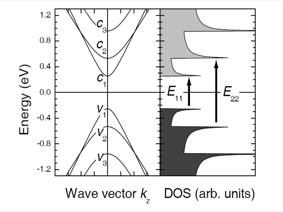
15 Van Hove szingularitás E

16

17 (17,0) cikk-cakk cső 2,4eV Félvezető

18 (18,0) cikk-cakk cső Fémes

19 (10,10) karosszék cső Fémes

20 (14,6) királis cső Félvezető

21 (16,1) királis cső Fémes

22

23 11 22 Kataura plot

24 (a) Kataura plot: transition energies of semiconducting (filled symbols) and metallic (open) nanotubes as a function of tube diameter. (Calculated from the Van-Hove singularities in the joint density of states within the third-order tight-binding approximation.) (b) Expanded view of the Kataura plot highlighting the systematics in (a). The optical transition energies follow roughly 1/d for semiconducting (black) and metallic nanotubes (grey). The V-shaped curves connect points from selected branches (2n+m = 22, 23 and 24). For each nanotube subband transition E ii it is indicated whether the ν = −1 or the +1 family is below or above the 1/d average trend. Squares (circles) are zigzag (armchair) nanotubes.

25 K M  n=3i n=3i+1 x 1/d n mod 3 = 2n mod 3 = 0n mod 3 = 1 n=3i+2 triad structure of zigzag tubes (due to trigonal warping)

26 K trigonal warping

27 Lines of allowed k vectors for the three nanotube families on a contour plot of the electronic band structure of graphene (K point at center). (a) metallic nanotube belonging to the ν = 0 family (b) semiconducting −1 family tube (c) semiconducting +1 family tube Below the allowed lines the optical transition energies E ii are indicated. Note how E ii alternates between the left and the right of the K point in the two semiconducting tubes. The assumed chiral angle is 15◦ for all three tubes; the diameter was taken to be the same, i.e., the allowed lines do not correspond to realistic nanotubes.

28 Kis átmérőjű szén nanocsövek (görbületi effektusok)

29 MOTIVÁCIÓ  Lehetővé vált kis átmérőjű nanocsövek előállítása: - HiPco ( 0.8 nm) - CoMocat ( 0.7 nm) - DWNTs, borsók (peapods) melegítésével ( 0.6 nm) - növesztés zeolit csatornákban ( 0.4 nm)  FELMERÜLŐ KÉRDÉS: A KIS ÁTMÉRŐJŰ CSÖVEK TULAJDONSÁGAI (geometria, sávszerkezet, rezgési frekvenciák stb) KÖVETIK-E A NAGY ÁTMÉRŐJŰ CSÖVEKÉT? grafénból „zónahajtogatás”-sal NEM

30 M. J. Bronikowski et al., J. Vac. Sci. Technol. A 19, 1800 (2001) High-Pressure CO method (HiPco) diameter down to  0.7 nm

31 peapods double-walled carbon nanotubes heating S.Bandow et al., CPL 337, 48 (2001) inner tube diameter down to  0.5 nm

32 SWCNT in zeolite channel (AFI)(d SWCNT  0.4 nm) picture from Orest Dubay J.T.Ye, Z.M.Li, Z.K.Tang, R.Saito, PRB 67 113404 (2003) O Al or P

33 FIRST PRINCIPLES CALCULATIONS DFT: LDA plane wave basis set, cutoff: 400 eV G. Kresse et al Wien Budapest Lancaster

34 arrangement: tetragonal (hexagonal for test) distance between tubes: l = 0.6 nm (1.3 nm for test) hexa tetra

35 r1r1 r2r2 r3r3 11 22 33 bond lengths bond angles (4,2) d c 56 atoms building block

36 tube axis ideal hexagonal lattice

37 tube axis d increases c decreases

38 tube axis extra bond misalignment 11

39 GEOMETRY OPTIMIZATION

40 diameter

41 1/d vs 1/d 0 DFT optimized diameter 1/d 0 (nm -1 ) 1/d (nm -1 ).  ZZ  AC  CH r 0 = 0.1413 nm

42 (d-d 0 )/d 0 vs 1/d 0 relative change 1/d 0 (nm -1 ) (d-d 0 )/d 0 (%).  ZZ  AC  CH r 0 = 0.1413 nm (9,0) : 1.06 ± 0.01 %

43 (d-d 0 )/d 0 vs 1/d 0 relative change 1/d 0 (nm -1 ) (d-d 0 )/d 0 (%).  ZZ  AC  CH r 0 = 0.1413 nm (9,0) : 1.06 ± 0.01 %

44 length of the unit cell

45 unit cell lengths vs 1/d 0 relative change 1/d 0 (nm -1 ) (c-c 0 )/c 0 (%).  ZZ  AC  CH r 0 = 0.1413 nm ZZ triads (9,0) : -0.05 ± 0.01 %

46 bond lengths

47 (r 1 -r 0 )/r 0 vs 1/d relative change 1/d (nm -1 ) (r 1 -r 0 )/r 0 (%).  ZZ  AC  CH r 0 = 0.1413 nm ZZ triads (9,0) : -0.32 ± 0.004 %

48 (r 2 -r 0 )/r 0 vs 1/d relative change 1/d (nm -1 ) (r 2 -r 0 )/r 0 (%).  ZZ  AC  CH r 0 = 0.1413 nm ZZ triads

49 bond angles

50 bond angle  1 vs 1/d 0 DFT optimized 1/d 0 (nm -1 )  1 (deg).  ZZ  AC  CH r 0 = 0.1413 nm

51 pyramidalization or  rehybridization sp 2 sp 3 S.Niyogi et al., Acc. Chem. Res. 35, 1105 (2002)

52 pyramidalization angle  P vs 1/d DFT optimized 1/d 0 (nm -1 )  P (deg)  ZZ  AC  CH r 0 = 0.1413 nm C 60 : 11.6°

53 SÁVSZERKEZET

54 TB vs DFT sávszerkezet (10,10)

55 (6,5) - DFT

56 (20,0) zigzag chiral (19,0) (17,0) (16,0) (14,0) (13,0) (11,0) (10,0) (8,0) (7,0)(5,0)(4,0) (6,4) (6,2) (5,3) (6,1) (4,3) (5,1) (4,2) (3,2) ZF-TB DFT  1/d

57     ZF-TB: E g = 2.3 eV DFT: E g = 0 ! (5,0) királis cső fémes

58 (20,0) zigzag chiral (19,0) (17,0) (16,0) (14,0) (13,0) (11,0) (10,0) (8,0) (7,0)(5,0)(4,0) (6,4) (6,2) (5,3) (6,1) (4,3) (5,1) (4,2) (3,2) ZF-TB DFT  1/d

59 ZF-TB METALLIC non-armchair: zigzag, chiral kFkF  k F  k F - k F (d  ) = f(1/d 2 ) K tube axis Másodlagos gap megjelenése

60 Másodlagos gap a (6,3) csőben

61 secondary gap in (7,1) 0.14 eV

62 Nagyobb átmérőn nincs ilyen

63 ZF-TB METALLIC armchair  k F  k F - k F (d  ) = f(1/d 2 ) K kFkF tube axis Nincs másodlagos gap

64 (6,6) (4,4) k F (d  )=2/3 kFkF kFkF FF FF

65 AC (3,3) (4,4) (5,5) (6,6) (7,7) (8,8) (9,9) (10,10) (11,11)